Summer Smackdown - Week 1

Published

July 7, 2019

These posts will most likely wind up being a bit of an odd bunch in terms of formatting until I figure out a style I like and enjoy, as the goal is to merge all Four of the lessons into one big post.

Given I wanted to update all of these blogs on Sundays, I decided I would include the first ‘day’ of work as well.

Overall how the schedule I plan to follow looks is as such:

M: Linear Algebra
T: NLP, Matrix Calculus
Th: Foundations, Matrix Calculus, Linear Algebra
F: Foundations, NLP
Sa: NLP, Linear Algebra, Matrix Calc, Foundations

As I started this goal on a Saturday, this week there will not be much in my recap, but I’ll be as inclusive as I can into the small lessons I learned.

Computational Linear Algebra

We start off learning about the Markov Chain, a way to describe a sequence of events where the probably of each event depends on the state of the previous event. Also known as the next event is determined by the previous event. The course utilizes the Numpy library to hold matrix multiplications to solve the various problems. My notes go through and futher explain what each answer means in context.

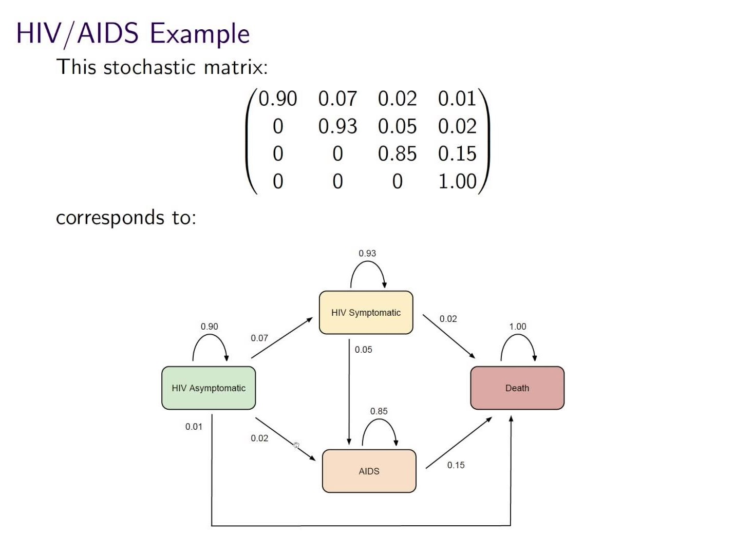
For example, problem 1 is about using a stochastic matrix, which is a square probablity matrix, in order to predict how health-related incidents will be in the following year.

We start off knowing that the current year had 85% asymtpmatic, 10% symptomatic, 5% AIDS, and 0% death. Next, we were given the following probability table:

Now that we’re here, we use matrix multiplication to get our answer:

import numpy as np

i = np.array([[.85,.1,.05,0]])
mat = np.array([[.9,.07,.02,.01],
                [0,.93,.05,.02],
                [0,0,.85,.15],
                [0,0,0,1]])

res = mat.T @ i.T

The @ symbol is used when doing matrix multiplication, where we multiply each row by the column, and then sum them together.

One thing Jeremy points out is another way to write the above:

(i @ mat).T) which saves us a few seconds of code, and looks cleaner.

The answer winds up being:

array([[0.765 ],
       [0.1525],
       [0.0645],
       [0.018 ]])

However, what does the answer mean? Well, it means that within the next year:

76.5% of people will be asymptomatic
15.25% of people will be symptomatic
6.45% of people will have AIDS
1.8% of people will die as a result of their illnesses

We’ve started using some matrix multiplication to get solutions, but can we get a bit more advanced with it?

Take problem 2:

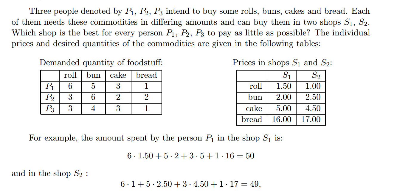
Given the above table, figure out which store is best for what individual. This is a straight matrix by matrix multiplication problem where we will have ‘dem’ represent a matrix of the demand per individual, and ‘p’ be the prices for each item in two particular shops.

dem = np.array([[6, 5, 3, 1],
       [3,6,2,2],
       [3,4,3,1]])

p = np.array([[1.5, 1],
       [2., 2.5],
       [5., 4.5],
       [16., 17.]])

We yet again solve this by doing dem@p, which gives us a table that looks like the following:

array([[50. , 49. ],
       [58.5, 61. ],
       [43.5, 43.5]])

The above table is now described as having the rows be an individual, and the columns being a particular store with the content as the price they would pay for the items they need. We can see that for Person 1 shop 2 would be the best, for Person 2 shop 1 would be the best, and for Person 3 they could go to either one.

Then Rachel goes further to describe images a little bit and convolutions, which I was already familar with from the Practical Deep Learning for Coders course, however this Medium article she mentions I found especially helpful: CNNs from Different Viewpoints

What this helped show for me was how matrix multiplication is actually applied within these Neural Networks we are generating through the Fast.AI library, especially the following image:

Here we have a 2x2 matrix (filter) being applied on a single-channel image (3x3), to get our four results: P,W,R,S. I enjoy this view of how our layers are working as I can see each product mapped with corresponding coordinates, versus a Neural Network viewpoint: 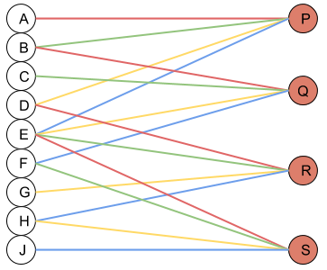alt text

Where alpha, beta, gamma, etc are the connections or lines from each node to result.

This is as far as I got yesterday, so next week lesson 1 should be fully completed.

Matrix Calculus

One thing Jeremy suggests us to do during the Foundations course is turn paper to code, so I wanted to apply that to this course, despite it being pure-math heavy. The goal of doing this was just to know how to apply various scary-looking math into code easier, as my experience before this was none.

This week I went over the Introduction and Review sections of the paper, as I last took AP Calculus senior year of high school… It’s been a few years.

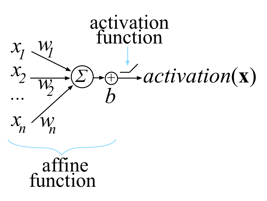
So! The introduction segment. Any activation of a single unit inside a nerual network is done using the “dot product of an edge weight vector, w, with an input vector x, plus a scalar bias b.” Okay. That was a lot thrown out at me. Let’s make that a bit easier. The above can also be written as y=mx+b, a basic linear function where m and x are both matrix’s. The better way to right that would be like so:

Where n and i are how many layers or activation uits we have. This could then also be written as z = w * x + b where z, the ‘affine function’ (linear function), is derived from a linear unit that clips negative values to zero from the bias.

Another way to visualize a neuron is like so:

Now, when we are training our models, all we are doing is choosing a w and b so we can get our desired output for all of our inputs. We can help choose and navigate what are our best options by using a loss function to grade the final activations to the target for all of our inputs. To help minimize, a variation of gradient decent is used where we take the partial derivitive (gradient) of an activation with respect to w and b.

In laymans terms? Gradually tweaking w and b in order to make some loss function as close to zero as we can.

The next example shown in the paper is taking a function we’re familair with, Mean Squared Error, and showing us its derivitive (gradient): alt text

At first glance that looks absolutely disgustingly terrifying. But let’s try to break it down into code instead and see if we can try to understand it better.

So first, the original where N is the number of inputs

def loss(N):
  y = 0
  for x in range(N):
    y += (targ(x) - activ(x)) ** 2
  return y/N

Okay, doesn’t look too bad now. For all inputs, we take the square of our target minus our activation (or our answer). Let’s look at that derivitive now. I made two functions, actf and grad as we have that interior summation.

def grad(N, w, b):
  y = 0
  for x in range(N):
    y += (targ(x) - actf(x)) ** 2
  return y/N

def actf(x, w, b):
  y = 0
  for i in range(abs(x)):
    y += (w[i] * x[i] + b)
  return max(0, y)

That looks a bit better, we can see that w and x are both going to be matrix’s, weight and input respectivly, and b is our bias.

Alright, not as scary anymore. The last bit I did was a review on the Scalar derivative rules, and attempting to recreate this in code. For this I found the sympy library a huge help, as we can visualize functions and their derivitives.

For example, say I have the equation

We can write this in code as y = 3*x**2. Well, if we want the derivitive all we have to do is first declare ‘x’ as a ‘Symbol’, then use the .diff function to get the derivitive!


from sympy import *
x = Symbol('x')
y = 3*x**2
yprime = y.diff(x)

The result will give us 6*x, what we were expecting.

Natural Language Processing

As I stated before, this course is not quite done yet, so as a result I’m going through the notebooks carefully to learn what I can and once the videos are released I will be rewatching them to make sure I did not miss anything and I understand all the concepts. But for now, here’s what I’ve learned:

There are many ethical issues that are brought upon by NLP’s, such as Google Translate:

Here we can see the same translation does not keep the proper pronouns as it should, and is bias towards men being doctors, not very 21st Century if you ask me!

But, onwards we must go. The topics I went into this week were on using Non-Negative Matrix Factorization (NMF) and Single Value Decomposition (SVD) for Topic Modeling. Topic modeling beings with something called a term-document matrix, which is a matrix of words by material. In the example used, we have the amount of times particular names showed up in a few classic books:

This is called a bags of words approach as we don’t care for the sentence structure or order words come in, just how often they appear.

For this lesson, Rachel used the Newsgroups dataset which consists of 18,000 blog posts that follow 20 topics on a forum, this was popular in the 80’s and 90’s apparently as the internet did not exist really then.

From here, we went into a few topics: stop words, stemming, and lemmatization

Stop Words:

Stop words are ‘extremely common words which are of little value in helping’. There is no single universal list of stop words, and each program uses a slightly different one. For example,the sklearn library has the following first twenty as theirs:

from sklearn.feature_extraction import stop_words
sorted(list(stop_words.ENGLISH_STOP_WORDS))[:20]
['a',
 'about',
 'above',
 'across',
 'after',
 'afterwards',
 'again',
 'against',
 'all',
 'almost',
 'alone',
 'along',
 'already',
 'also',
 'although',
 'always',
 'am',
 'among',
 'amongst',
 'amoungst']

These words are usually ignored and dropped, however for Machine Learning its been found recently that we (ML algorithms) may benefit more from their inclusion than exclusion.

Stemming and Lemmatization:

Stemming and lemmatization are used to generate the root forms of words. Lemmatization uses the rules of the original language, thus the tokens are all actually words. In contrast, stemming just chops the ends off of the words. These results won’t be actual words, but it is faster. “Stemming is the poor-man’s lemmatization” (Noah Smith, 2011).

To visualize this, we can use the nltk library. Say we have a list of words: organize, organizes, organizing. We know that they all stem from organize in some degree or another. Let’s compare the two together. We can do this with the following code:

 import nltk
 from nltk import stem
 wl = ['organize', 'organizes', 'organizing']
 [wnl.lemmatize(word) for word in wl]
 [porter.stem(word) for word in wl]

The output of this code is radically different:

Lemmatization: [‘organize’, ‘organizes’, ‘organizing’]

Stemming: [‘organ’, ‘organ’, ‘organ’]

Lemmatization will allow us to have more context within the words we tokenize and is almost always better than using Stemming, especially with languages that have more compex morphologies.

The last topic I got through in the lesson was Spacy. Spacy is a modern and fast NLP library, which Fast.AI uses. Spacy always uses Lemmatization for it’s tokenizations, as it is considered better. This is the first example of an opinionated choice in a library.

I did not get into Foundational course yet this week, so I won’t have an update on that until the following post, but thank you all for reading! The goals for the upcoming week for each course are:

NLP: Finish topic modeling
Matrix Calculus: Introduction to vector calculus and partial derivatives
Linear Algebra: Finish the ‘Why are we here’ notebook and the NMF SVD Notebooks
Foundations: Get through notebooks 01 and 02

See you next week!

Zach Mueller